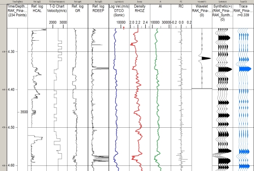
Synthetic seismogram from a well in deepwater Nigeria.
Proper display should always:
1.- start with the caliper curve (tells the audience how reliable are the logs),
2.- continue with the display of the time-depth table the synthetic is using,
3.- show essential geologic logs i.e. SP/GR and resistivity
(tells the audience something about the geology),
4.- clearly display the sonic and density logs the synthetic is based on
5.- show the Acoustic impedance curve (AI)
(tells the audience how the seismic data sees the gerology)
6.- show the reflection coefficient curve (tells the audience where
prominent soft kicks and hard kicks will be,
7.- show the wavelet (essential that it has the same bandwith, polarity and phase
as the field seismic data,
9.- show a trace extracted from the field seismic data at the well in blue
10.- show a scale on the left or right, showing both time and depth.
In this case, the sonic and density logs required some editing for washouts prior to modeling.
The two hydrocarbon-bearing sands (resistivity spikes) clearly show as zones of
low impedance on the AI curve. In the upper sand, there is a clear impedance increase
at the base of the gas, while he base of the sand soes not show an impedance change.
It can already be predicted at this point that the hydrocarbon-water contact will be
a strong hard kick, while the top and base of the formation will only have a weak
seismic signature. When the wavelet is applied (normal North American polarity),
the HWC is demostrated by a strong hard kick (black), which ties very well with
a hard kick on the field seismic (blue). The base of the formation is not seen on seismic.
The top of the formation is associated with a weak soft kick on the RC series,
but due to the limited bandwidth of the wavelet (and of the seismic data), it is not imaged.
